Before we Start

Overview

Teaching: 15 min
Exercises: 10 min

Questions

• How to find your way around RStudio?

• How to interact with R?

• How to manage your environment?

• How to install packages?

Objectives

• Install latest version of R.

• Install latest version of RStudio.

• Navigate the RStudio GUI.

• Install additional packages using the packages tab.

• Install additional packages using R code.

R and RStudio

R is an open source programming language originally designed and implemented by statisticians primarily for statistical analysis. It includes high quality graphics capabilities and tools for data analysis and reading and writing data to/from files.

Because R is open source and is supported by a large community of developers and users, there is a very large selection of third-party add-on packages which are freely available to extend R’s native capabilities.

R is a scripted language. Rather than pointing and clicking in a graphical environment, you write code statements to ask R to do something for you. This has the advantage of providing a record of what was done and allowing for peer review of the work undertaken. Having this written record, something which is increasingly required as part of a publication submission, is also an aid when seeking help with problems.

There are many online resources, such as stackoverflow and the RStudio Community, which will allow you to seek help from peers. Questions which are backed up with short, reproducible code snippets are more likely to attract knowledgeable responses.

To make it easier to interact with R, we will use RStudio. RStudio is the most popular IDE (Integrated Development Interface) for R. An IDE is a piece of software that provides tools to make programming easier.

A tour of RStudio

Knowing your way around RStudio

Let’s start by learning about RStudio, which is an Integrated Development Environment (IDE) for working with R.

The RStudio IDE open-source product is free under the Affero General Public License (AGPL) v3. The RStudio IDE is also available with a commercial license and priority email support from RStudio, Inc.

We will use the RStudio IDE to write code, navigate the files on our computer, inspect the variables we create, and visualize the plots we generate. RStudio can also be used for other things (e.g., version control, developing packages, writing Shiny apps) that we will not cover during the workshop.

One of the advantages of using RStudio is that all the information you need to write code is available in a single window. Additionally, RStudio provides many shortcuts, autocompletion, and highlighting for the major file types you use while developing in R. RStudio makes typing easier and less error-prone.

Getting set up

It is good practice to keep a set of related data, analyses, and text self-contained in a single folder called the working directory. All of the scripts within this folder can then use relative paths to files. Relative paths indicate where inside the project a file is located (as opposed to absolute paths, which point to where a file is on a specific computer). Working this way makes it a lot easier to move your project around on your computer and share it with others without having to directly modify file paths in the individual scripts.

RStudio provides a helpful set of tools to do this through its “Projects” interface, which not only creates a working directory for you but also remembers its location (allowing you to quickly navigate to it). The interface also (optionally) preserves custom settings and open files to make it easier to resume work after a break. Below, we will go through the steps to create an “R Project” for this tutorial. First, let’s take a quick tour of RStudio.

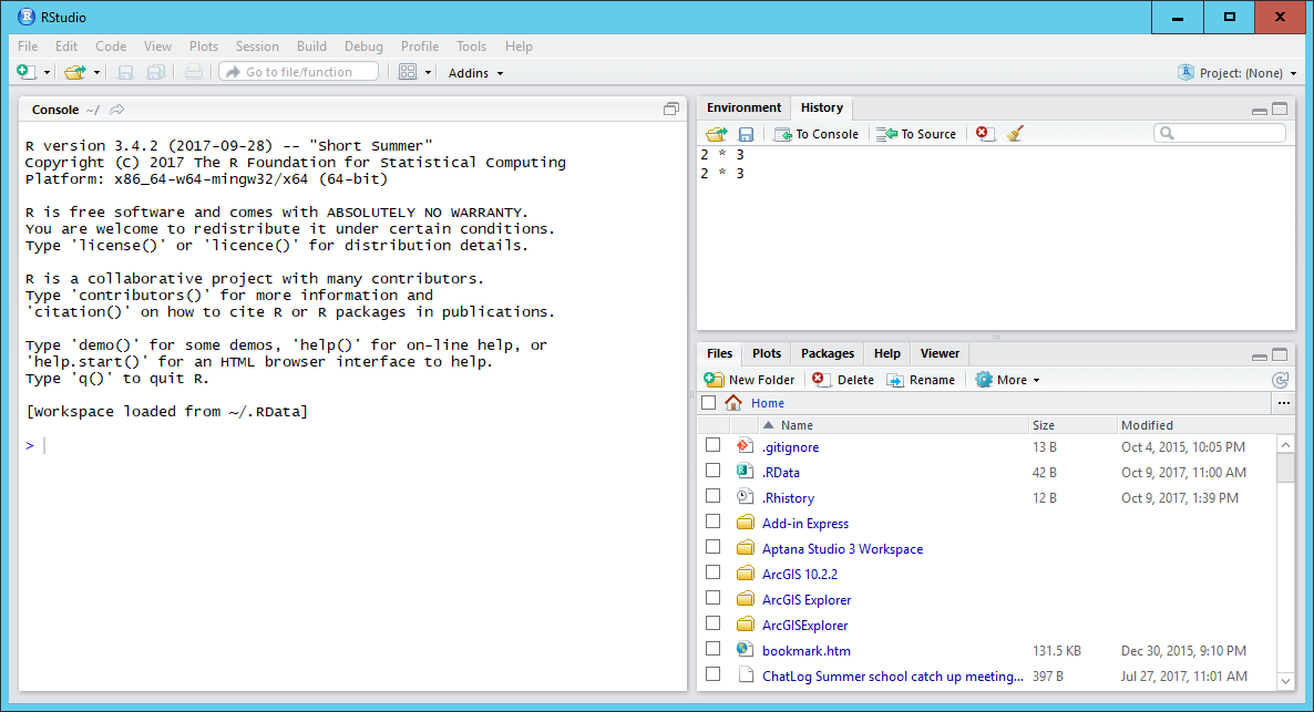
RStudio is divided into four “panes”: the Source for your scripts and documents (top left in the default layout), the R Console (bottom left), your Environment/History (top right), and your Files/Plots/Packages/Help/Viewer (bottom right). The placement of these panes and their content can be customized (see menu, Tools -> Global Options -> Pane Layout).

Create a new project

• Under the File menu, click on New project, choose New directory, then New project
• Enter a name for this new folder (or “directory”) and choose a convenient location for it. This will be your working directory for the rest of the day (e.g., ~/ltrc-workshop)
• Click on Create project
• Create a new folder called scripts. In the console, type dir.create(scripts), You should see a folder in the bottom right window called scripts.
• Create a new file where we will type our scripts. Go to File > New File > R script. Click the save icon on your toolbar and save your script as “script.R”.

Organizing your working directory

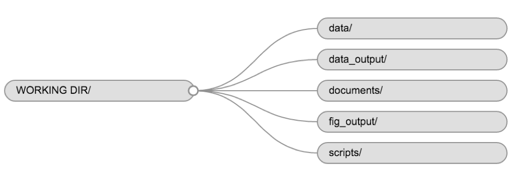
Using a consistent folder structure across your projects will help keep things organized and make it easy to find/file things in the future. This can be especially helpful when you have multiple projects. In general, you might create directories (folders) for scripts, data, and documents. Here are some examples of suggested directories:

• data/ Use this folder to store your raw data and intermediate datasets. For the sake of transparency and provenance, you should always keep a copy of your raw data accessible and do as much of your data cleanup and preprocessing programmatically (i.e., with scripts, rather than manually) as possible.
• data_output/ When you need to modify your raw data, it might be useful to store the modified versions of the datasets in a different folder.
• documents/ Used for outlines, drafts, and other text.
• fig_output/ This folder can store the graphics that are generated by your scripts.
• scripts/ A place to keep your R scripts for different analyses or plotting.

You may want additional directories or subdirectories depending on your project needs, but these should form the backbone of your working directory. Use the dir.create function to create the other folders.

The working directory

The working directory is an important concept to understand. It is the place where R will look for and save files. When you write code for your project, your scripts should refer to files in relation to the root of your working directory and only to files within this structure.

Using RStudio projects makes this easy and ensures that your working directory is set up properly. If you need to check it, you can use getwd(). If for some reason your working directory is not what it should be, you can change it in the RStudio interface by navigating in the file browser to where your working directory should be, clicking on the blue gear icon “More”, and selecting “Set As Working Directory”. Alternatively, you can use setwd("/path/to/working/directory") to reset your working directory. However, your scripts should not include this line, because it will fail on someone else’s computer.

Downloading the data and getting set up

For this workshop we will use the following folders in our working directory: data/, data_output/, fig_output/, documents, and scripts. Let’s write them all in lowercase to be consistent. We can create them using the RStudio interface by clicking on the “New Folder” button in the file pane (bottom right), or directly from R by typing at console:

dir.create("data")
dir.create("data_output")
dir.create("documents")
dir.create("fig_output")
# dir.create("scripts") # we have already done this; doing it again would erase what we have created in the current folder

The data for this workshop can all be found at its GitHub repository https://github.com/gtlaflair/ltrc-2019/data. You can download it directly to your computer by running the commands below in R or RStudio. The names in all of the datasets are fake; they were generated using the charlatan package from rOpenSci.

download.file("https://raw.githubusercontent.com/gtlaflair/ltrc-2019/gh-pages/data/placement_1.csv",
              "data/placement_1.csv", mode = "wb")

download.file("https://raw.githubusercontent.com/gtlaflair/ltrc-2019/gh-pages/data/placement_2.csv",
              "data/placement_2.csv", mode = "wb")

download.file("https://raw.githubusercontent.com/gtlaflair/ltrc-2019/gh-pages/data/integrated.csv",
              "data/integrated.csv", mode = "wb")

Interacting with R

The basis of programming is that we write down instructions for the computer to follow, and then we tell the computer to follow those instructions. We write, or code, instructions in R because it is a common language that both the computer and we can understand. We call the instructions commands and we tell the computer to follow the instructions by executing (also called running) those commands.

There are two main ways of interacting with R: by using the console or by using script files (plain text files that contain your code). The console pane (in RStudio, the bottom left panel) is the place where commands written in the R language can be typed and executed immediately by the computer. It is also where the results will be shown for commands that have been executed. You can type commands directly into the console and press Enter to execute those commands, but they will be forgotten when you close the session.

Because we want our code and workflow to be reproducible, it is better to type the commands we want in the script editor and save the script. This way, there is a complete record of what we did, and anyone (including our future selves!) can easily replicate the results on their computer.

RStudio allows you to execute commands directly from the script editor by using the Ctrl + Enter shortcut (on Mac, Cmd + Return will work). The command on the current line in the script (indicated by the cursor) or all of the commands in selected text will be sent to the console and executed when you press Ctrl + Enter. You can find other keyboard shortcuts in this RStudio cheatsheet about the RStudio IDE.

At some point in your analysis, you may want to check the content of a variable or the structure of an object without necessarily keeping a record of it in your script. You can type these commands and execute them directly in the console. RStudio provides the Ctrl + 1 and Ctrl + 2 shortcuts allow you to jump between the script and the console panes.

If R is ready to accept commands, the R console shows a > prompt. If R receives a command (by typing, copy-pasting, or sent from the script editor using Ctrl + Enter), R will try to execute it and, when ready, will show the results and come back with a new > prompt to wait for new commands.

If R is still waiting for you to enter more text, the console will show a + prompt. It means that you haven’t finished entering a complete command. This is likely because you have not ‘closed’ a parenthesis or quotation, i.e. you don’t have the same number of left-parentheses as right-parentheses or the same number of opening and closing quotation marks. When this happens, and you thought you finished typing your command, click inside the console window and press Esc; this will cancel the incomplete command and return you to the > prompt. You can then proofread the command(s) you entered and correct the error.

Installing additional packages using the packages tab

In addition to the core R installation, there are in excess of 10,000 additional packages which can be used to extend the functionality of R. Many of these have been written by R users and have been made available in central repositories, like the one hosted at CRAN, for anyone to download and install into their own R environment. In the course of this lesson we will be making use of several of these packages, such as ‘ggplot2’ and ‘dplyr’.

Additional packages can be installed from the ‘packages’ tab. On the packages tab, click the ‘Install’ icon and start typing the name of the package you want in the text box. As you type, packages matching your starting characters will be displayed in a drop-down list so that you can select them.

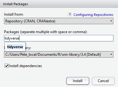
At the bottom of the Install Packages window is a check box to ‘Install’ dependencies. This is ticked by default, which is usually what you want. Packages can (and do) make use of functionality built into other packages, so for the functionality contained in the package you are installing to work properly, there may be other packages which have to be installed with them. The ‘Install dependencies’ option makes sure that this happens.

Exercise

Use the install option from the packages tab to install the ‘tidyverse’ package.

Solution

From the packages tab, click ‘Install’ from the toolbar and type ‘tidyverse’ into the textbox, then click ‘install’. The ‘tidyverse’ package is really a package of packages, including ‘ggplot2’ and ‘dplyr’, both of which require other packages to run correctly. All of these packages will be installed automatically. Depending on what packages have previously been installed in your R environment, the install of ‘tidyverse’ could be very quick or could take several minutes. As the install proceeds, messages relating to its progress will be written to the console. You will be able to see all of the packages which are actually being installed.

Because the install process accesses the CRAN repository, you will need an Internet connection to install packages.

It is also possible to install packages from other repositories, as well as Github or the local file system.

Installing additional packages using R code

There are a few packages that we forgot to ask you to install before coming today. We will do that now. We will explain what these packages do as we use them.

install.packages(c('here', 'skimr'))

Key Points

• Use RStudio to write and run R programs.

• Use install.packages() to install packages (libraries).