Part 5: Reproducible Reporting
Overview
Teaching: 40 min
Exercises: 35 minQuestions
Can I use Rmarkdown to create research reports
How do I automate score reporting?
How do I combine my analysis and reporting?
Objectives
Create a research report.
Write a command that will print score reports for your test takers.
Create a presentation that includes code, prose, and results.
The purpose of this part of the workshop is to illustrate how R and RStudio can be leveraged to create a reproducible pipeline for analysis and reporting. Some of the parts in this section move beyond analysis. We will spend just enough time with them to grasp the basics.
There are quite a few R packages that have been created to promote reproducible research. Some of these packages are tools for accessing databases, some are tools for managing projects, and others are tools for creating reproducible reports. A couple of groups, RStudio and ROpenSci, and people affiliated (officially and unofficially) with them have led the way in this. Today, the main packages that we will be using to learn about this are knitr, rmarkdown, tinytex, and xaringan. knitr is an “engine for dynamic report generation with R”, rmarkdown is a “file format for making dynamic documents with R”, and tinytex is a subset of packages from a larger distribution of LaTeX. This last package we will use first and only once to install the $\LaTeX$ distribution on your computer. It makes creating PDF documents easier.
tinytex::install_tinytex()
We will interact with knitr primarily through the button in RStudio and through the use of its kable function to create tables.
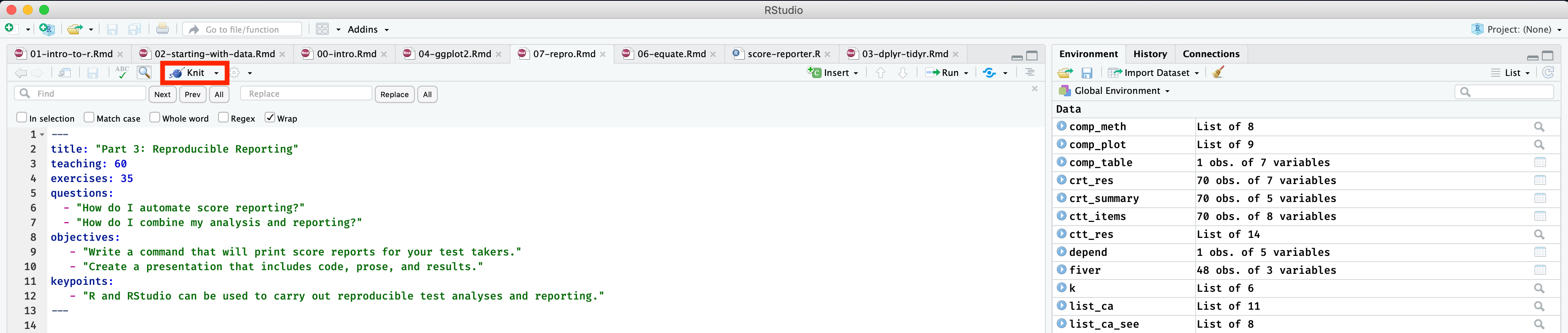
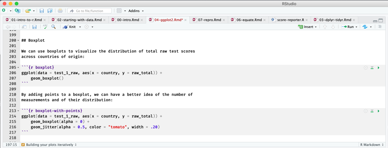
You can think of an rmarkdown file, or an .Rmd, file in the same way you think of a .docx file. A place to do writing. Writing in a .Rmd file differs in that you can include R code in your writing, and you do not do heavy formatting in the file. Below is an example of R chunks (in grey) embedded in prose (we saw this code and this prose in the lesson on data visualization). The “chunks” start with backticks followed by {r} and they end in three backticks. The chunks can be named, and there are parameters that can be set globally across chunks or specifically for one chunk such as fig.width to control the width of figures and echo to indicate the printing of code with results or not. The gray area is like a mini-environment for R code. You can write and run R code inside of it. When you click the “knit” button, it will compile a document for you that knits together your prose and the ouputs of your analyses.
Research reports
Now, we will work on creating a research report. There are a lot methods for doing this that range from “quick and easy” to more complicated with more formatting options (e.g. the papaja package for creating APA manuscripts). We are going to work with the quick and easy method :).
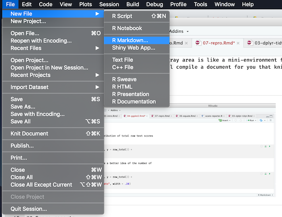
To start a .Rmd file go to File > New file > Rmarkdown. Save it in the documents folder. Let’s also start a new .R file for this part (file.create('scripts/report.R'))
Rmarkdown documents have a third component beyond code and prose: yaml. Yaml stands for Yaml ain’t a markup language. It is found at the top of the document sandwiched between --- at the top and --- at the bottom. This can be used to set parameters for the document and add information such as the title, data, and author (depending on the type of document you are making). You can start a .Rmd through the File menu in Rstudio:
Let’s save this file as report.Rmd in the documents folder. First we will compile it as is so that we can see how the knit button works. Some example minimal, inline formating that can be done is below. More can be found on RStudio’s Rmarkdown cheatsheet.
# Level 1 Header
## Level 2 Header

- unordered list
- unordered list
  + nesting


1. ordered list
2. item 2
   i) sub-item 1
     A. sub-sub-item 1

Markdown table

| Right | Left | Default | Center |
|------:|:-----|---------|:------:|
| 12|12| 12 | 12|
| 123 | 123 | 123 | 123 |
| 1 | 1 | 1 | 1 |
Now, let’s make some changes. Let’s read in some of our data, make a table, and a plot:
# read in data
library(tidyverse)

test_results_1 <- here::here("data/placement_1.csv") %>%
  read_csv()

# select read and listen main idea items
test_res_an <- test_results_1 %>%
  select(., contains('list'), contains('read')) %>%
  select(contains('_mi')) %>%
  summarise_all('mean')


# tables by skill

list_diff <- select(test_res_an, contains('_list_')) %>%
  knitr::kable(., digits = 2, caption = 'Listening: Main idea item difficulties')
read_diff <- select(test_res_an, contains('_read_'))%>%
  knitr::kable(., digits = 2, caption = 'Reading: Main idea item difficulties')

list_diff
| q1_list_mi | q10_list_mi | q12_list_mi | q20_list_mi | q23_list_mi | q30_list_mi_an | q31_list_mi_an |
|---|---|---|---|---|---|---|
| 0.61 | 0.77 | 0.62 | 0.35 | 0.36 | 0.7 | 0.81 |
list_diff
| q1_list_mi | q10_list_mi | q12_list_mi | q20_list_mi | q23_list_mi | q30_list_mi_an | q31_list_mi_an |
|---|---|---|---|---|---|---|
| 0.61 | 0.77 | 0.62 | 0.35 | 0.36 | 0.7 | 0.81 |
# visualize

list_read_mi <- test_res_an %>%
  gather(key, value = Difficulty) %>%
  separate(key, into = c('Question', 'Skill', 'Objective', 'Anchor'), sep = "_", fill = 'right')%>%
  ggplot(., aes(x = Question, y = Difficulty, color = Difficulty)) +
  geom_errorbar(aes(x = Question, ymin = Difficulty, ymax = Difficulty), size = 2) +
  facet_wrap(~ Skill, scales = 'free_x') +
  scale_color_viridis_c()

list_read_mi

Presentations
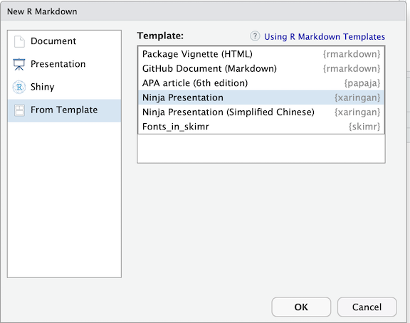
There are quite a few frameworks for creating presentations in R (ioslides, Rpres, beamer). One of the more developed and supported (with documentation and in the user community) is xaringan. This package is hosted on GitHub rather than the official R repository, CRAN. You can install the package by copying or typing the devtools::install_github('yihue/xaringan'). An easy way to start building a presentation using this platform is also through the dropdown menu. However, instead of selecting an option from the Document group, you will select “From Template” then “Ninja Presentation”.
The beauty of Rmarkdown and these code chunks is that you can use them in different document types. So if we copy our code from above into a xaringan file, we can easily make the same tables and plots in the presentation. Often, I will do all of the coding in a .R file, read that file in at the top of my presentation or paper, and call on the objects I want to print.
Score reports
In order to generate individual score reports for test takers, we need an R script (.R file) that has reads in the data and does some summarizing prior to the reporting. We also need a .Rmd file that serves as a template for the score reports. Doing the calucations in the R script makes it so these calculations are done once and then used in the reporting code, rather than done for each student (which would happen if they were in the .Rmd). Both can be downloaded using the download.file command below. Or you can copy and pase the R code below into an .R file.
download.file("https://raw.githubusercontent.com/gtlaflair/ltrc-2019/gh-pages/_episodes_rmd/documents/score-report-template.Rmd",
              "documents/score-report-template.Rmd", mode = "wb")
download.file("https://raw.githubusercontent.com/gtlaflair/ltrc-2019/gh-pages/_episodes_rmd/scripts/score-reporter.R",
              "scripts/score-reporter.R", mode = "wb")
#load packages
library(tidyverse)
library(rmarkdown)
library(knitr)

#load data
test_results_2 <- here::here('data/placement_2.csv') %>%
  read_csv(.)

#compute total and part scores
test_results_2 <- test_results_2 %>%
  mutate(total = rowSums(.[5:69], na.rm = TRUE),
         list_total = rowSums(select(., contains('_list_')), na.rm = TRUE),
         read_total = rowSums(select(., contains('_read_')), na.rm = TRUE))

#compute mean, save these values
total_mean <- mean(test_results_2$total, na.rm = TRUE)
list_mean <- mean(test_results_2$list_total, na.rm = TRUE)
read_mean <- mean(test_results_2$read_total, na.rm = TRUE)


# select a subset so that we do not waste time making 100 score reports today
test_results_rep <- slice(test_results_2, 1:5)

for (i in unique(test_results_rep$ID)){
  student <- test_results_rep %>% filter(ID == i)
  doc_path <- here::here('documents/')
  here::here('documents/score-report-template.Rmd') %>%
  rmarkdown::render(., output_file = paste0(doc_path, 'Score_Report_', as.character(student$names),'.pdf'))
}
Key Points
Rmarkdown provides a flexible framework for analysis and reporting.
R and RStudio can be used to carry out reproducible test analyses and reporting.