Part 4: Test Equating
Overview
Teaching: 30 min
Exercises: 20 minQuestions
How do I prepare data for test equating?
How do I conduct test equating?
How do I extract indices of interest for comparison, reporting, and analysis?
how do I visualize equated relationships?
Objectives
Prepare frequency tables of test scores.
Use
equateto conduct equating studies.Extract estimates of error for presenting in figures.
We start by loading the required packages.
library(tidyverse)
library(equate)
If not still in the workspace, load the data we saved in the previous lesson. We also need to calculate the raw total and raw anchor scores for the reading and listening tests,
# load test_1_raw_totals
test_1_raw <- read_csv('data_output/test_1_raw_totals.csv') %>% # read in our total score data from earlier
  select(-country)

# load placement 1 and 2 data
test_results_1 <- read_csv('data/placement_1.csv')

test_results_2 <- read_csv('data/placement_2.csv')

# create total raw and anchor scores
test_2_raw <- test_results_2 %>%
  mutate(raw_total = rowSums(.[5:69], na.rm = TRUE)) %>%
  mutate(read_raw_total = rowSums(select(., contains("_read_")), na.rm = TRUE)) %>%
  mutate(list_raw_total = rowSums(select(., contains("_list_")), na.rm = TRUE)) %>%
  mutate(list_an_raw = rowSums(select(., matches("q\\d+_list_\\w{2,4}_an")), na.rm = TRUE)) %>% # ugly regex for summing listening anchor items
  mutate(read_an_raw = rowSums(select(., matches("q\\d+_read_\\w{2,4}_an")), na.rm = TRUE)) %>%
  select(ID, contains('raw'))

# write_csv(test_2_raw, 'data_output/test_2_raw_totals.csv')
Preparing the data
The equate function requires frequency tables of the test scores that are to be equated. We
are working with data that was collected under the Non-equivalent group anchor test (NEAT) design.
As a result, we need bivariate frequency tables, or frequency tables of score combinations on the
anchor and total test. The equate package has a function named freqtab to help us compute these.
We will be using two arguments in this function: x and scales. We will start with the listening
test.
One quick way for us to figure our how many items are on the total test and how many are on the
anchor test is to select the columns of the items and then count them:
listen_1_total_q <- test_results_1 %>%
  select(contains('list'))

listen_1_an_q <- test_results_1 %>%
  select(contains('list')) %>%
  select(contains('an'))

ncol(listen_1_total_q)
[1] 35
ncol(listen_1_an_q)
[1] 9
listen_1_freq <- freqtab(test_1_raw[c('list_raw_total', 'list_an_raw')], scales = list(0:35, 0:9))
Exercise
Figure out the total and anchor scales for the
test_2_rawdata and then create a frequency table for it.Solution
# How many questions are on the total and anchor forms?
listen_2_total_q <- test_results_2 %>%
  select(contains('list'))

listen_2_an_q <- test_results_2 %>%
  select(contains('list')) %>%
  select(contains('an'))

ncol(listen_2_total_q)
[1] 30ncol(listen_2_an_q)[1] 9# Create the frequency table listen_2_freq <- freqtab(test_2_raw[c('list_raw_total', 'list_an_raw')], scales = list(0:30, 0:9))
Now that we have the frequency tables, we are ready to equate. There are a number of consderations in choosing an equating method Kolen & Brennan’s Test Equating, Scaling, and Linking is a nice resource for those of you who want to take a deep dive into it.
We will use the circle-arc method right now to equate form 1 on to scores from form 2:
list_ca <- equate(listen_1_freq, listen_2_freq, type = 'circle-arc', lowp = c(0, 0), highp = c(35, 30))
Exercise
What does a score of 32 on form 1 concord to on form 2? (hint:
strorglimpse)Solution
list_ca$concordancescale yx 1 0 0.0000000 2 1 0.3920108 3 2 0.8166926 4 3 1.2729186 5 4 1.7596900 6 5 2.2761212 7 6 2.8214275 8 7 3.3949150 9 8 3.9959714 10 9 4.6240594 11 10 5.2787099 12 11 5.9595173 13 12 6.6661353 14 13 7.3982727 15 14 8.1556914 16 15 8.9382033 17 16 9.7456691 18 17 10.5779963 19 18 11.4351392 20 19 12.3170976 21 20 13.2239176 22 21 14.1556914 23 22 15.1125584 24 23 16.0947067 25 24 17.1023745 26 25 18.1358527 27 26 19.1954879 28 27 20.2816857 29 28 21.3949150 30 29 22.5357132 31 30 23.7046926 32 31 24.9025471 33 32 26.1300615 34 33 27.3881212 35 34 28.6777250 36 35 30.0000000
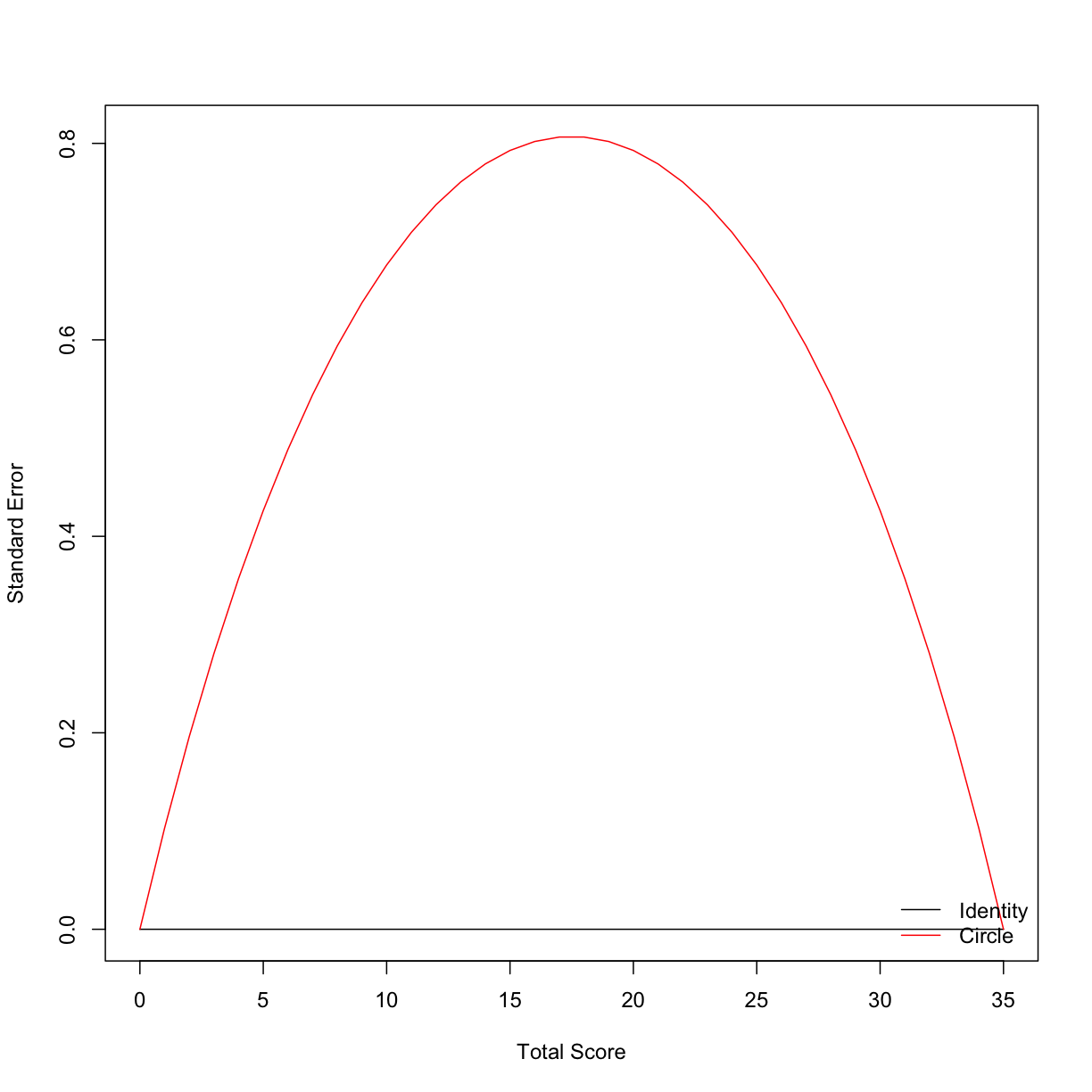
There are three types of error associated with equating: random error, systematic error (or bias), and total error. To calculate the latter two, we would need a criterion, or gold standard, equating relationship between the two test forms that we could compare our circle-arc methods to. We dont have that, so we will estimate the standard error by bootstrapping the equating relationship. One way to inspect the random error is by plotting it:
list_ca_see <- bootstrap(list_ca, reps = 100)

list_ca_see$se
 [1] 3.071556e-15 1.028392e-01 1.960803e-01 2.805879e-01 3.570847e-01
 [6] 4.261793e-01 4.883871e-01 5.441462e-01 5.938296e-01 6.377548e-01
[11] 6.761917e-01 7.093678e-01 7.374740e-01 7.606676e-01 7.790755e-01
[16] 7.927970e-01 8.019048e-01 8.064469e-01 8.064469e-01 8.019048e-01
[21] 7.927970e-01 7.790755e-01 7.606676e-01 7.374740e-01 7.093678e-01
[26] 6.761917e-01 6.377548e-01 5.938296e-01 5.441462e-01 4.883871e-01
[31] 4.261793e-01 3.570847e-01 2.805879e-01 1.960803e-01 1.028392e-01
[36] 3.071556e-15
plot(list_ca_see, out = 'se')

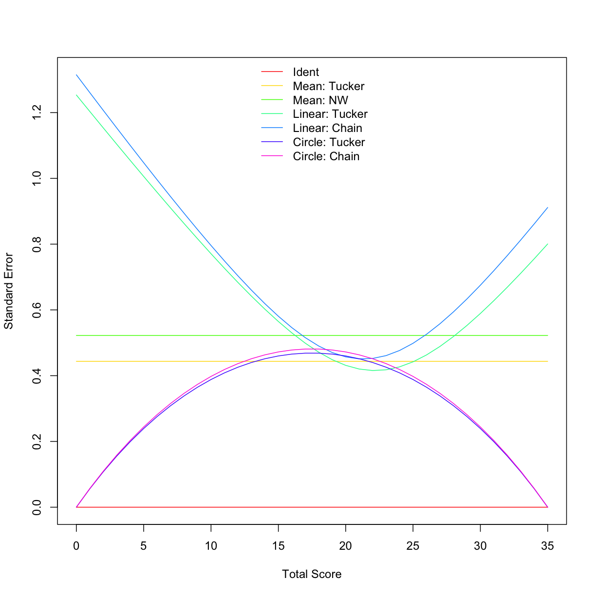
Usually, in carrying out a full equating study, multiple equating relationships are estimated and compared. Below is a demonstration of how this can be done in a few lines of code.
neat_args <- list(identity = list(type = "identity"),
                  mean_tuck = list(type = "mean", method = "tucker"),
                  mean_nomi = list(type = "mean", method = "nominal weights"),
                  line_tuck = list(type = "linear", method = "tucker"),
                  line_chai = list(type = "linear", method = "chained"),
                  circ_tuck = list(type = "circle-arc", method = "tucker"),
                  circ_chai = list(type = "circle-arc", method = "chained", chainmidp = "linear"))

comp_meth <- bootstrap(x = listen_1_freq, y = listen_2_freq, reps = 100, args = neat_args)

plot(comp_meth, out = "se", addident = FALSE, legendplace = 'top')

round(summary(comp_meth), 2)
            se se_w
identity  0.00 0.00
mean_tuck 0.44 0.44
mean_nomi 0.52 0.52
line_tuck 0.74 0.54
line_chai 0.78 0.58
circ_tuck 0.34 0.40
circ_chai 0.35 0.41
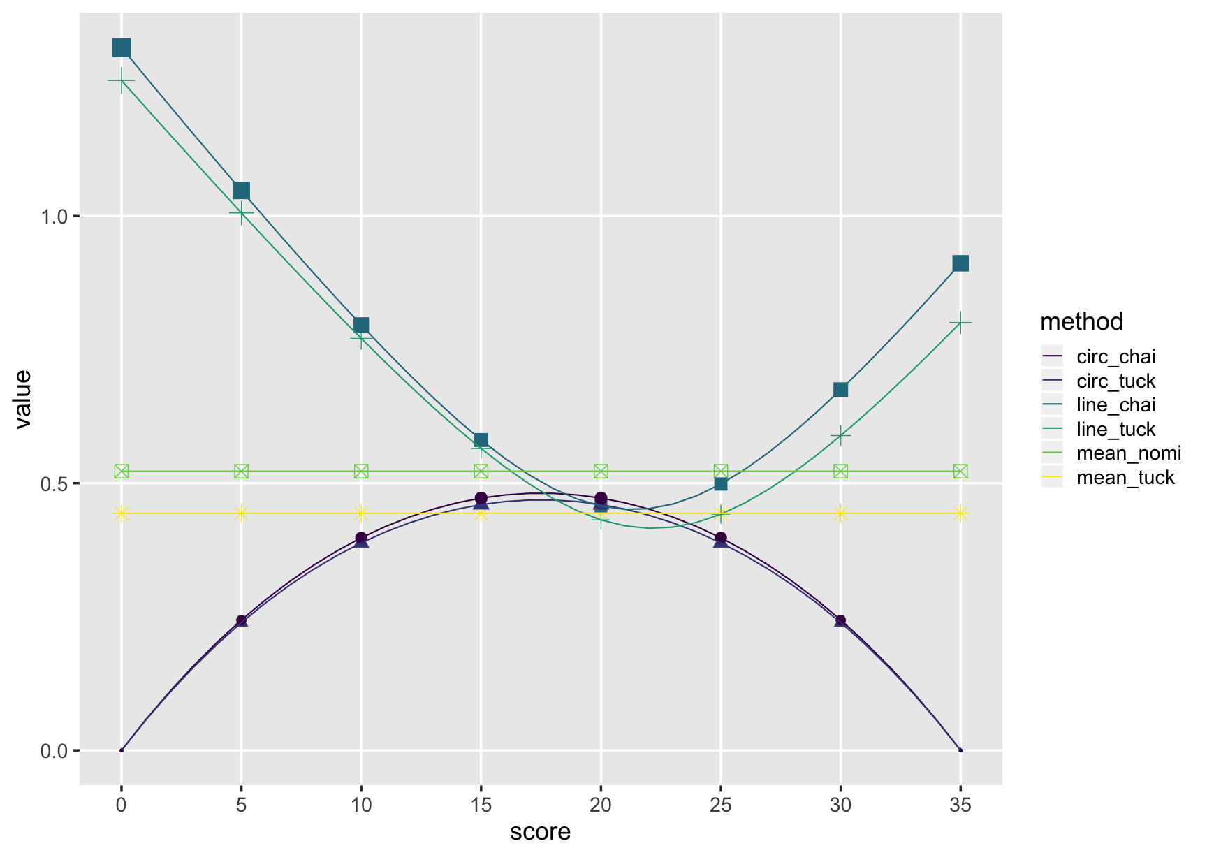
# using ggplot and dplyr/tidyr

fiver <- comp_meth$se %>%
  as_tibble() %>%
  select(-identity) %>%
  mutate(score = 0:35) %>%
  slice(seq(1, 36, by = 5)) %>%
  gather(key = method, value, -score)

comp_plot <- comp_meth$se %>%
  as_tibble() %>%
  select(-identity) %>%
  mutate(score = 0:35) %>%
  gather(key = method, value, -score) %>%
  ggplot(., aes(x = score, y = value, colour = method, shape = method)) +
  geom_point(data = fiver, aes(size = value), show.legend = FALSE) +
  geom_line() +
  theme_gray(base_size = 18) +
  scale_colour_viridis_d() +
  scale_x_continuous(breaks = c(0, 5, 10, 15, 20, 25, 30, 35), limits = c(0, 35)) +
  theme(panel.grid.minor = element_blank())

comp_plot

comp_table <- comp_meth$se %>%
  as_tibble() %>%
  summarise_all(., 'mean') %>%
  mutate_all(., 'round', 2)

comp_table
# A tibble: 1 x 7
  identity mean_tuck mean_nomi line_tuck line_chai circ_tuck circ_chai
     <dbl>     <dbl>     <dbl>     <dbl>     <dbl>     <dbl>     <dbl>
1        0      0.44      0.52      0.69      0.74      0.31      0.32
Key Points
equatecan be used for small- and large-sample test equating.